常用的一些算法

建议使用黑色主题

常用库

1
2
3
4
import numpy as np
import matplotlib.pyplot as plt
import matplotlib as mpl
import scipy as sp

1 数值计算的根本概念

1.1 浮点数的存储方法:

$A = 1.5 = 2 * 0.75 = 2 * (0.5+0.25)= 2^{1} * (2{-1}+2{-2} ) $

符号位 指数位 尾数位
1 00000001 1100~~
1
2
3
4
5
6
7
8
9
10
11
12
13
14
15
16
17
18
19
20
21
22
23
24
25
26
27
28
#这是一个把浮点数变成float32储存字节的算法
def trans_to_byte(A):
if A >= 0 :
symbol = "1"
else:
symbol = "0"
print("符号位:",symbol)
A = abs(A)
count = 0
while A > 1:
A = A /2
count+= 1
exp = ""
for i in range(8-len(bin(5).split("0b")[1])):
exp = exp+"0"
exp += bin(count).split("0b")[1]
print("指数位:",exp)
remain = ""
for i in range(1,24):
if A-2**(-i)>=0:
remain = remain + "1"
A = A - 2**(-i)
else:
remain = remain + "0"
A = A
print("尾数:",remain)
return(symbol+exp+remain)
trans_to_byte(-0.55)
符号位: 0
指数位: 000000
尾数: 10001100110011001100110
'000000010001100110011001100110'

1.2 python的机器精度测试

1
2
3
4
5
6
a = 1
count = 0
while 1 + a > 1:
a = a/10
count += 1
print(count)
16

可知python的机器精度在\(10^{-16}\)左右,机器精度可以理解为所能存储和操作的最小的数的单元,但是一般计算涉及不到那么小的舍入误差,

避免方法有:

1.避免过于临近的数相减

2.减少运算次数

3.尽量选取合适的单位制使得乘除法的数字在1附近

4.有一些递推算法,类似于待求值\(S_n=a*S_{n-1},a>1\)这种,会不断放大舍入误差,也不可取

2 函数求值

2.1 泰勒展开

\(f(x)= \frac{sin(x)}{x}\)类的函数在奇点(0)附近,由于舍入误差的原因,会出现不规则的震荡,这会儿需要用解析的方法对函数进行近似

1
2
3
4
5
x = np.linspace(1e-20,1e-15,10000)
y = [np.sin(i)/i for i in x]
%matplotlib inline
plt.plot(x,y)
plt.show()

numpy应该已经处理过这个问题了

\(f(x) = \frac{sinx}{x}=\frac{x-\frac{x^3}{3!}...}{x} = 1 - \frac{x^2}{3!}...\)

1
2
3
4
5
x = np.linspace(1e-16,1e-15,10000)
y = [1-i**2/np.math.factorial(3) for i in x]
%matplotlib inline
plt.plot(x,y)
plt.show()

级数求解与阶乘求解

一般为了简化求解,\((x -x_0)^k\)\((x-x_0)^{k-1}\)生成,并且一般会做截断,同时阶乘会化成ln和exp的形式

\[ e^{0.5} = \sum_{i}{\frac{(0.5-0)^i}{i!}}, ln(i!) = \sum_{1}^i ln(n) \]

1
2
3
4
5
6
7
8
9
10
11
12
print(np.exp(0.5))
diff_x = 0.5 - 0
fact_ln = 0
diff_x_n = (0.5-0)**0
result = diff_x_n/1
for i in range(1,121):
fact_ln += np.log(i)
factorial_n = np.exp(fact_ln)#ln,exp生成阶乘
diff_x_n = diff_x_n*diff_x#递推生成递推公式
result += diff_x_n/factorial_n

print(result)
1.6487212707001282
1.6487212707001278

3 数值计算的根本概念

3.1 迭代法求根

迭代法求\(x^2-5x+4=0\)的根,迭代公式为\(x_n = \frac{x_{n-1}^2~~+4}{5}\)

1
2
3
4
5
6
7
8
9
10
11
12
13
14
15
16
17
def solve_eq(x, re_fun, tol,init_point = 1): 
step = 0
if init_point == 1 and type(x) != list:
x = [x,re_fun([x])]
step = 1 #手动算了一个点
def distance(x):
return np.abs(x[-1]-x[-2])

while (distance(x) > tol):
x.append(re_fun(x))
step += 1
return x,step

def fun_iteration(x):
return (x[-1]**2+4)/5

solve_eq(2,fun_iteration,1e-5)
([2,
  1.6,
  1.312,
  1.1442688,
  1.061870217330688,
  1.0255136716907844,
  1.010335658164943,
  1.0041556284319177,
  1.0016657052223,
  1.0006668370036975,
  1.000266823735797,
  1.0001067437333,
  1.000042699772165,
  1.0000170802735202,
  1.0000068321677553,
  1.0000027328764378],
 15)

收敛条件:

\(g'(x)\mid_\{x_{n}\}<1\)时一定收敛,也就是初值点和迭代点落在\(|g'(x)|<1\) 的区间内

prove:

\(g(x)\)代表迭代公式:

\[\begin{aligned} &x_{i+1}-x_{i} = g(x_{i}) - g(x_{i-1}) = g(\epsilon)|x_i-x_{i-1}| \\\\ &if ~ g(\epsilon) <1 \Rightarrow x_{i+1}-x_{i}< |x_i-x_{i-1}| \end{aligned}\]

所以所有迭代过程中取值范围内的迭代公式的导数值都小于1,迭代恒收敛(实际上还与迭代方向有关,若迭代反向,导数值迟早大于1,也有可能实际并没有解)

牛顿迭代法:\(x_{n+1} =x_{n}-f(x_n)/f'(x_n)\)

此时\(f(x) = x^2-5x+4\)

1
2
3
def fun_newton(x):
return x[-1]-(x[-1]**2-5*x[-1]+4)/(2*x[-1]-5)
solve_eq(2,fun_newton,1e-10)
([2,
  0.0,
  0.8,
  0.9882352941176471,
  0.9999542229343099,
  0.9999999993015081,
  1.0,
  1.0],
 7)

弦截法:(用差商代替微商):\(x_{n+1} =x_{n}-f(x_n)\frac{x_k-x_{k-1}}{f(x_k)-f(x_{k-1})}\)

1
2
3
4
5
def f(x):
return x**2-x*5+4
def fun_string(x):
return x[-1]-(x[-1]-x[-2])/(f(x[-1])-f(x[-2]))*f(x[-1])
solve_eq([2,1.8],fun_string,1e-10,init_point = 2)
([2,
  1.8,
  0.33333333333333526,
  1.1860465116279069,
  1.0356347438752782,
  0.9976137655897542,
  1.000028661939602,
  1.0000000227801336,
  0.9999999999997824,
  1.0],
 8)

4 函数插值

4.1 拉格朗日插值

\(\phi(x) = y_0 l_0(x)+ y_1 l_1(x) + y_2 l_2(x) + y_3 l_3(x)...\)

\(l_i(x) = \frac{(x-x_0)(x-x_1)...(x-x_n)}{(x_i-x_0)(x_i-x_1)..(x_i-x_n)}\)

插目标函数:\(f(x) = e^{2x} - x^2\)

1
2
3
4
5
6
7
8
9
10
11
12
13
14
15
16
17
18
19
20
21
22
23
24
25
26
27
28
29
30
31
32
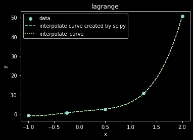
# scipy的拉格朗日插值
from scipy.interpolate import lagrange
x=np.linspace(-1,2,5)
y = np.exp(2*x)-x**2
poly = lagrange(x, y)
x1 = np.linspace(-1,2,1000)

#手算的插值
def lagrange_dyf(x,y,x_target):
result = 0
component = list()
for i in range(len(x)):
tem = 1
#计算第n个插值多项式
for j in range(0,i):
tem *= (x_target - x[j])/(x[i] - x[j])
for j in range(i+1,len(x)):
tem *= (x_target - x[j])/(x[i] - x[j])
tem *= y[i]
result += tem
return result

%matplotlib inline
fig, ax = plt.subplots(1)
plt.scatter(x,y,label ="data")
plt.plot(x1,[poly(i) for i in x1],label = r"interpolate curve created by scipy",linestyle = "--")
plt.plot(x1,[lagrange_dyf(x,y,i) for i in x1],label = r"interpolate_curve",linestyle = ":")
ax.legend(); # Add a legend.
ax.set_xlabel('x') # Add an x-label to the axes.
ax.set_ylabel('y') # Add a y-label to the axes.
ax.set_title("lagrange") # Add a title to the axes.
plt.show()
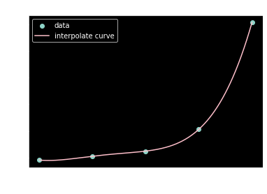
4.2 牛顿插值

插值表达式为:

\[\begin{equation} \begin{aligned} p(x) &= f[x_0](x-x_0) + f[x_0,x_1](x-x_0)(x-x_1) \\&+ f[x_0,x_1,x_2](x-x_0)(x-x_1)(x-x_2)... \end{aligned} \end{equation}\]

优势在于便于扩展,每次多一个数据点,不用重新算插值系数和插值基,同时插值基的大小顺序没有关系,插值系数有对称性。

1
2
3
4
5
6
7
8
9
10
11
12
13
14
15
16
17
18
19
20
21
22
23
24
25
26
27
28
29
30
31
32
def Newton_interpolate_dyf(x,y,x_target):
func = dict(zip(x,y))
def get_ceff(X): # 得到 f[x0,x1,x2..xn]的函数,X是一个[x0,x1,x2,..xn]的列表
if len(X)==1 :
return func[X[0]]
else:
return (get_ceff(X[1:len(X)]) - get_ceff(X[0:len(X)-1]))/(X[-1]-X[0])
result = 0
for i in range(0,len(x)):
# print('在算第'+str(i+1)+'个项,系数为',x[0:i+1])
poly = 1
for j in range(0,i):
poly *= x_target-x[j]
# print("多",poly,x[i],x_target)
result += get_ceff(x[0:i+1])*poly
#print(result)
return result

x=np.linspace(-1,2,5)
y = (np.exp(2*x)-x**2).tolist()
x = x.tolist()
x1 = np.linspace(-1,2,1000)

%matplotlib inline
fig, ax = plt.subplots(1)
plt.scatter(x,y,label ="data")
plt.plot(x1,[Newton_interpolate_dyf(x,y,i) for i in x1],label = r"interpolate curve",color = "pink")
ax.legend(); # Add a legend.
ax.set_xlabel('x') # Add an x-label to the axes.
ax.set_ylabel('y') # Add a y-label to the axes.
ax.set_title("Newton") # Add a title to the axes.
plt.show()

5 数值积分

5.1 简单积分方法:梯形积分

积分公式:

\[ T = \sum_{i}{(f(x_i)+f(x_{i+1}))\frac{\Delta x_i}{2}} \]

误差分析:

某一个矩形积分区间中:

\[\begin{aligned} &T_{theory} - T_{numerical} = F(x_{i+1})-F(x_i) - (f(x_i)+f(x_{i+1}))\frac{\Delta x_i}{2} \\\\ &= F'(x_i) \Delta x_i +\frac{1}{2}F''(x_i) \Delta x_i ^2 + \frac{1}{6}F'''(x_i)\Delta x_i ^3 - f(x_i)\Delta x_i \\\\&- \frac{1}{2} f'(x_i)\Delta x_i ^2 -\frac{1}{4}f''(x_i)\Delta x_i ^3 \\\\ &= \frac{1}{12} f''(x_i) \Delta x_i ^3 \end{aligned}\]

\(F(x)\)\(f(x)\) 的原函数,第二行来源于在\(x_{i+1}\)的泰勒展开,所以将所有梯形分区的误差加一起后得到最大误差上限\((b-a)\frac{w^3}{12}M\)\(M\)为f(x)导数区间的最大值,w是分割长度,b,a,积分上下限

物理中常用的积分与求和相互转换 \(\int_a^b f(x)dx = \frac{(b-a)}{N}\sum_i^N f(x_i),x_i = a+\frac{b-a}{N} i= \sum_i^N f(x_i) \Delta V\),转换成了求面积

1
2
3
4
5
6
7
8
9
10
11
12
13
#f(x) = sin(x) a = 0 ,b = pi
def intergrate_Trapezoid(func,a,b,N):
x = np.linspace(a,b,N)
w = (b-a)/N
y = [func(i) for i in x]
T = 0
for i in range(len(x)-1):
T += (y[i] + y[i+1])*w/2
return T
print(intergrate_Trapezoid(np.sin,0,np.pi,100000))

import scipy.integrate as integrate
print(integrate.quad(np.sin,0,np.pi))
1.9999799998355314
(2.0, 2.220446049250313e-14)

5.2 辛普森积分公式

推导:

由三点插值的拉格朗日插值公式:

\[\begin{aligned} p(x) =& f(x_0) \frac{(x-x_1)(x-x_2)}{(x_0-x_1)(x_0-x_2)} \\\\& + f(x_1) \frac{(x-x_0)(x-x_2)}{(x_1-x_0)(x_1-x_2)} \\\\&+ f(x_2) \frac{(x-x_0)(x-x_1)}{(x_2-x_0)(x_2-x_1)} \end{aligned}\]

\(x_1\)\(x_0\)\(x_2\)的中点,计算\(\int^{x_2}_{x_0}p(x)dx\)为:

\[ I = \frac{x_2-x_0}{6}[f(x_0)+4f(x_1)+f(x_2)] \]

误差分析方法同上,就不写了

1
2
3
4
5
6
7
8
9
10
11
12
def intergrate_simpson(func,a,b,N):
x = np.linspace(a,b,N)
w = (b-a)/N
T = 0
for i in range(len(x)-1):
T += (func(x[i])+4*func((x[i]+x[i+1])/2)+func(x[i+1]))*w/6
return T

print(intergrate_simpson(np.sin,0,np.pi,1000000))

import scipy.integrate as integrate
print(integrate.quad(np.sin,0,np.pi))
1.9999980000000428
(2.0, 2.220446049250313e-14)

高阶积分公式及隆贝格积分略

5.3 高斯积分公式

可以用多项式去插值对应的待积分函数,并且通过变量代换变到\([-1,1]\)的区间上通过几个关键的函数点(高斯点)对插值的多项式进行求解。

以两点高斯积分为例:

\[\begin{aligned} &p(-\frac{1}{\sqrt{3}})+ p(\frac{1}{\sqrt{3}}) = \int^1_{-1} p(x) dx \\\\&p(x) = ax^3+bx^2+cx+d \end{aligned}\] 则求积分的思路变为:
\(\int^b_a f(x)dx = \sum^{i} \int^{x_i+w}_{x_i}f(x)dx\)

\(= \sum^{i} \int^{1}_{-1}\frac{w}{2} f(\frac{w}{2}x'+x_i+\frac{w}{2})dx'\)

\(\approx \sum_{i} \frac{w}{2}(f(\frac{w}{2}\frac{1}{\sqrt 3}+x_i+\frac{w}{2})+f(-\frac{w}{2}\frac{1}{\sqrt 3}+x_i+\frac{w}{2}))\)
1
2
3
4
5
6
7
8
9
10
11
12
13
14
15
16
17
18
19
20
21
22
from scipy.special import roots_legendre #用于得到对应的高斯点 

def integrate_gauss(func,a,b,N):
x = np.linspace(a,b,N)
w = (b-a)/N
T = 0
for i in range(len(x)-1):
T += w/2*(func(w/2/np.sqrt(3)+x[i]+w/2)+func(-w/2/np.sqrt(3)+x[i]+w/2))
return T
print(integrate_gauss(np.sin,0,np.pi,100000))

def integrate_gauss_n(func,a,b,N,n):#n是高斯点的个数
x = np.linspace(a,b,N)
w = (b-a)/N
T = 0
x_gauss,a = roots_legendre(n) # scipy可以方便得到高斯点w以及对应的权重a
for i in range(len(x)-1):
for j in range(len(x_gauss)):
T += a[j]*w/2*func(w/2*x_gauss[j]+x[i]+w/2)
return T
print(integrate_gauss_n(np.sin,0,np.pi,100000,5))

1.9999799999999983
1.9999800000000323

5.4 反常积分的求解

5.4.1 解析处理

换元法对奇点降阶,(小于1阶的都可以)

\[ \int^{\frac{\pi}{2}}_0 \frac{f(x)}{\sqrt x} dx = \int^{\sqrt \frac{\pi}{2}}_0 \frac{f(x(u))}{u} 2u du \]

如果积分两端都是奇点,可以将区间分割成两部分分别求解,用分布积分等处理

5.2.分布积分

\(\int_{\epsilon}^a f(x)/x dx\)型的,$^{}_{x}f(x) \(,因为积分下限太小时可能算不准,需要将积分变形提出\)ln()$的表达式

\[\begin{aligned} \int_{\epsilon}^a \frac{sinx}{x^2}dx &= \int_{\epsilon}^a \frac{sinx/x}{x} dx \\\\&= \int_{\epsilon}^a \frac{sinx/x-1}{x} dx +\int_{\epsilon}^a \frac{1}{x} dx \\\\&= \int_{\epsilon}^{\delta} \frac{sinx/x-1}{x} dx + \int_{\delta}^a \frac{sinx/x-1}{x} dx \\\\&+ \ln(a) -\ln(\epsilon) \\\\&= \int_{\epsilon}^{\delta} \frac{1- 1 + \frac{1}{3!}x^3 - \frac{1}{5!}x^5 ..}{x} dx + \\\\&\int_{\delta}^a \frac{sinx/x-1}{x} dx + \ln(a) -\ln(\epsilon) \end{aligned}\]

若是有无穷区间的积分,不能简单截断,因为不能证明后面的积分是可忽略的量,而是要通过换元的方法去积分

有限离散傅里叶变换

f(t)是\([0,t_{end}]\)区间上的函数

变换公式:

\(F(w_n) = \sum^{N-1}_{l=0}f(t_l) e^{-i\frac{2\pi l}{N}}\)

\(f(t_l) = \sum^{N-1}_{k=0}F(w_n) e^{i\frac{2\pi n}{N}}\)

该变换主要用于频谱分析.需要的量为\(|{F(w_l)}|\),与傅里叶变换\(F(w_l)\)相比,该变换相差一个常数因子,见知乎回答

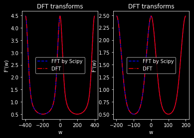
横坐标对应于\(w_l= \frac{2\pi l }{N\Delta t}\)\(\Delta t\)为取样间隔

将 $f(t) =e{-200t2} $ 做DFT变换

1
2
3
4
5
6
7
8
9
10
11
12
13
14
15
16
17
18
19
t_end = 1
N = 400 #不能少于两个点
t = np.linspace(0,2*np.pi*t_end,N)#是等距的点
delta_t = t[1] - t[0]
y = np.exp(-t**2*200)

def DFT_trans(f):#f是传入其中的采样点的np.array
F = list()
N = len(f)
for k in range(N):
tem = 0 #容器
for l in range(N):
tem += f[l]*np.exp(-1.j*k*2*np.pi*l/N)
F.append(tem)
return np.array(F)

import scipy.fft as fft
N = len(y)
#fft.fft(y)
1
2
3
4
5
6
7
8
9
10
11
12
13
14
15
16
17
18
19
20
21
22
23
24
25
26
27
28
29
30
31
w0 = np.linspace(-2*np.pi/delta_t,0,N)
w1 = np.linspace(0,2*np.pi/delta_t,N)
%matplotlib inline
fig, ax = plt.subplots(1,2)
#plt.scatter(x,y,label ="data")
ax[0].plot(w1,abs(fft.fft(y)),label = r"FFT by Scipy",color="blue",linestyle = "--")
ax[0].plot(w0,abs(fft.fft(y)),color="blue")
ax[0].plot(w0,abs(DFT_trans(y)),label = r"DFT",color="red",linestyle = "-.")
ax[0].plot(w1,abs(DFT_trans(y)),color="red")
ax[0].legend(); # Add a legend.
ax[0].set_xlabel('w') # Add an x-label to the axes.
ax[0].set_ylabel('F\'(w)') # Add a y-label to the axes.
ax[0].set_title("DFT transforms") # Add a title to the axes.

## 更改点数后再画
N = 200 #不能少于两个点
t = np.linspace(0,2*np.pi*t_end,N)#是等距的点
delta_t = t[1] - t[0]
y = np.exp(-t**2*200)
w0 = np.linspace(-2*np.pi/delta_t,0,N)
w1 = np.linspace(0,2*np.pi/delta_t,N)

ax[1].plot(w1,abs(fft.fft(y)),label = r"FFT by Scipy",color="blue",linestyle = "--")
ax[1].plot(w0,abs(fft.fft(y)),color="blue")
ax[1].plot(w0,abs(DFT_trans(y)),label = r"DFT",color="red",linestyle = "-.")
ax[1].plot(w1,abs(DFT_trans(y)),color="red")
ax[1].legend(); # Add a legend.
ax[1].set_xlabel('w') # Add an x-label to the axes.
ax[1].set_ylabel('F\'(w)') # Add a y-label to the axes.
ax[1].set_title("DFT transforms") # Add a title to the axes.
plt.show()

由于是\(f'(w)\)是周期函数,所以出现的峰值不一定就是正确的,需要更改取点数的多少从而更改w的范围从而更改\(f'(w)\)的周期来判断是不是真峰,没有移动的峰才是真峰,显然0点附近的高斯波包才是真峰。

矩阵求解之LU分解

若矩阵\(A=LU\),则求解\(Ax=b\)可转换成\(Ly=b\)再求解\(Ux = y\)\(L\)为下三角矩阵,\(U\)为上三角矩阵

Cholesky 分解

根据计算数学理论,一个正定对称矩阵一定可以做LU分解

由:

\[ \hat{A}_{ii} = \left( \begin{matrix} a_{ii}& \alpha\\\\ \alpha ^T& A_{i+1i+1} \end{matrix} \right) \]


\[ \,\,=\,\,\left( \begin{matrix} u_{ii}& 0\\\\ u^T& {U_{i+1i+1}}^T \end{matrix} \right) \left( \begin{matrix} u_{ii}& u\\\\ 0& U_{i+1i+1} \end{matrix} \right) \]

得到具体算法:

\[\begin{aligned} &u_{ii} = \sqrt{a_{11}} \\\\&u_{ij} = \frac{a_{ij}}{a_{ii}} \end{aligned}\]
\(\hat{A}_{i+1i+1}=U_{i+1i+1}^T U_{i+1i+1} = A_{i+1i+1}-u^Tu\)
1
2
3
4
5
6
7
8
9
10
11
12
13
14
def Cholesky_factorization(A):#A是对角正定矩阵
U = np.zeros(A.shape)
for i in range(0,A.shape[0]-1): #只用遍历到倒数第二行
U[i][i] = np.sqrt(A[i][i])
u_vec = A[i][i+1:A.shape[1]]/U[i][i]
tem = np.zeros(A.shape[1] - u_vec.shape[0]) # 用于对A操作,得到Ahat
u_vec = np.append(tem,u_vec)
A = A - np.outer(u_vec,u_vec) #将A hat用A右下角来储存
U[i] = U[i]+ u_vec
U[-1][-1] = np.sqrt(A[-1][-1])
return U
A = np.array([[3,-1,1],[-1,3,0],[1,0,3]])
print("U矩阵:\n",Cholesky_factorization(A))
print("L矩阵:\n",np.linalg.cholesky(A)) # numpy自带的分解
U矩阵:
 [[ 1.73205081 -0.57735027  0.57735027]
 [ 0.          1.63299316  0.20412415]
 [ 0.          0.          1.62018517]]
L矩阵:
 [[ 1.73205081  0.          0.        ]
 [-0.57735027  1.63299316  0.        ]
 [ 0.57735027  0.20412415  1.62018517]]

求解方程:

\[ \left[ \begin{matrix} 1& 3& 1\\\\ 3& 10& 4\\\\ 1& 4& 4\\\\ \end{matrix} \right] \left[ \begin{array}{c} x_1\\\\ x_2\\\\ x_3\\\\ \end{array} \right] =\\,\\,\left[ \begin{array}{c} 0\\\\ 2\\\\ -\frac{1}{3}\\ \end{array} \right] \]

1
2
3
4
5
6
7
8
9
10
11
12
13
14
15
16
17
18
19
20
21
22
23
A =np.array([[1,3,1],[3,10,4],[1,4,4]])
U = Cholesky_factorization(A)
L = U.transpose()
b = np.array([0,2,-1/3])
#先求解y
y = [b[0]/L[0][0]] #先把y1处理了
for i in range(1,len(b)):
tem = b[i]
for j in range(0,i):
tem = tem - L[i][j]*y[j]
tem = tem/L[i][i]
y.append(tem)
print("y:",y)
#求解x
x = np.zeros(len(y))
x[-1] = y[-1]/U[-1][-1]#先把y1处理了
for i in range(len(y)-1,-1,-1):
tem = y[i]
for j in range(len(y)-1,i,-1):
tem = tem - U[i][j]*x[j]
tem = tem/U[i][i]
x[i] = tem
print("x:",x)
y: [0.0, 2.0, -1.6499158227686108]
x: [-8.33333333  3.16666667 -1.16666667]
1
2
3
4
5
6
7
#numpy自带的求解线性方程组
y = np.linalg.solve(L,b)
print("y:",y)
x = np.linalg.solve(U,y)
print("x:",x)
x_prime = np.linalg.solve(A,b)
print("直接计算x:",x_prime)
y: [ 0.          2.         -1.64991582]
x: [-8.33333333  3.16666667 -1.16666667]
直接计算x: [-8.33333333  3.16666667 -1.16666667]

2. 高斯消去法得LU分解

假设\(A\)通过\(n\)次消去操作后变为上三角矩阵\(U\),既:

\[\begin{aligned} &L_1^{-1}..L_{n-1}^{-1}L_n^{-1}L_nL_{n-1}...L_1 A \\\\&= S (L_nL_{n-1}...L_1 A) = SU = A \\\\&S= L_1^{-1}..L_{n-1}^{-1}L_n^{-1} \end{aligned}\]

由消去操作对应的变换矩阵为下三角矩阵,且容易证明下三角矩阵的乘积仍然是下三角矩阵,可知S是下三角矩阵

同时容易证明\(S_{ij}= \frac{a_{ii}}{a_{ij}}\),通过矩阵的分量乘积表达式以及消去法的变换矩阵的特征易得

1
2
3
4
5
6
7
8
9
10
11
12
13
14
15
16
17
18
#假设是A是full pivoting的,也就是恰当排序使得在分解过程中不存在对角元为0的情况
def gauss_elimination_LU(A):
#a是系数矩阵,b是方程的非齐次值,a得满足一定条件,先将a分解成LU矩阵
N = A.shape[0]
L = np.identity(N)
for i in range(0,N):
if A[i][i] != 0:
for j in range(i+1,N):#消去
if A[i][j] != 0:
tem = A[i][j]/A[i][i]
A[j] = A[j] - tem*A[i]
L[j][i] = tem
else:
pass
else:
print("A不是恰当排序的")
return 0
return L,A

求解实矩阵的本征值

Householder变换

存在向量\(\left|w \right>\)\(\left|e_0 \right>\),欲找到映射\(H\),使得\(H \left|w \right> = ||w||\left|e_0 \right>\),这个映射被定义为Householder变换,容易验证:

\[\begin{aligned} H &= I - \frac{2\left| v\right>\left< v \right|}{\left< v|v \right>} \\\\v &= \left|w \right> \pm ||w||\left|e_0 \right> \end{aligned}\]

同时也容易验证\(HH = I,H^T = H\)

QR分解

矩阵\(A_0\)的第一行列向量为\(w\)\(e_0\)为矩阵的基矢量,则可以得到\(H_0A_0 = A_1\)\(A_1\)的第一行列向量除了00元都为0,再考虑\(U_1 = e_1 \oplus e_2...\oplus e_n\)空间以及\(A_1' = A_1 \mid_{U_1}\),同样的操作得到子空间上的\(H_1'A_1' = A_2'\)\(H_1'\)是子空间上的映射,在子空间的矩阵表达式中除了11元都为0,令\(H_1 e_i = H_1'e_i \enspace i>0, H_1 e_0 = e_0\),则可得到\(H_1H_0 A_0 = A_2\)\(A_2\)的前两列的下三角元都为0,同样的方法,最终\(n\)步后,得到上三角矩阵\(A_n\),以及\(H_nH_{n-1}...H_{0}A_0 = A_n\),再由\(H\)的性质得到\(A_0 = H_0H_1...H_nA_n\),于是得到正交矩阵\(Q=H_0H_1...H_n\)和上三角矩阵\(R = A_n\)

求解特征值

想要求实矩阵\(A_i\)的本征值,对\(A_i=QR\)做合同变换\(A_{i+1}=QQRQ^T = RQ\),则\(A_i\)的本征值全都相同,由一个数学理论可以得到,\(i\rightarrow \infty\)时,\(A_i\)趋近于上三角矩阵,再由上三角矩阵的对角元既为特征值

留一个我参考的文章

Notes on Householder QR Factorization 侵删

1
2
3
4
5
6
7
8
9
10
11
12
13
14
15
16
17
18
19
20
21
22
23
24
25
26
27
28
29
def QR_factorization(A):#为了简单,这里讨论实数矩阵
A = np.array(A,dtype=float)
N = A.shape[0]
Householder_Matrix = list()
for i in range(N-1): #来源于参考文献
#print(A[i:,i])
alpha = np.linalg.norm(A[i:,i])
signi = np.sign(A[i][i])
rho = -signi * alpha
nu1 = A[i][i] - rho
u2 = A[i+1:,i]/nu1
tau = (1 + np.dot(u2,u2))/2
#记录使用的Householder变换的矩阵
tem_matrix = np.identity(N,dtype = float)
tem_matrix[i:,i:] = np.identity(N-i) - np.outer(np.insert(u2,0,1),np.insert(u2,0,1))/tau
Householder_Matrix.append(tem_matrix)
#print(Householder_Matrix[-1])
#print(np.matmul(Householder_Matrix[-1],A))
#手动求解变换后的对角矩阵,减少矩阵运算的次数
A[i][i] = rho
for j in range(i+1,N):
A[j][i] = 0
w12T = (A[i,i+1:] + np.matmul(A[i+1:,i+1:],u2))/tau
A[i,i+1:] = A[i,i+1:] - w12T
A[i+1:,i+1:] = A[i+1:,i+1:] - np.outer(u2,w12T)
Q = np.identity(N)
for j in Householder_Matrix:
Q = np.matmul(Q,j)
return Q,A
1
2
3
4
5
6
7
8
9
10
11
12
13
14
A = np.array([[3,3,1],[3,5,2],[1,2,3]])
def get_eigen_values(A):#A是一个有特征值的实矩阵,没写判断条件,所以用的实对称矩阵检验
tol = 1
N = A.shape[0]
for i in range(0,10000):
tol = 0
Q,R = QR_factorization(A)
A = np.matmul(R,Q)
for i in range(0,N):
for j in range(N-1,i,-1):
tol += np.abs(A[j][i])
return np.array([A[i][i] for i in range(N)])
print(get_eigen_values(A))
np.linalg.eigvals(A)
[8.11753167 2.13093256 0.75153577]
array([8.11753167, 0.75153577, 2.13093256])

常用的一些算法
http://dyf.zone/2023/01/17/algorithm/
作者
Duyifei
发布于
2023年1月17日
许可协议